Gradient Descent for Linear Regression

I was searching for something(I do not remember) and I saw below post.
GradientDescentExample

This was a perfect post to test some parameters on gradient descent.
I opened my databricks notebook and began to play with it. I took the functions from this page but changed a bit
because of type changes in my code.

Question : Check picture below. We have points as below, is there a formula
that identifies this spread.

I used y1 = 5 * x1 + 10 + noise formula to generate this data.
So our target values are 5 and 10. ( Or a little different because of noise)

noise = np.random.normal(-3, 6, 49)

x1 = np.linspace(0, 50, 49)
y1 = 5 * x1 + 10 + noise
points = zip(x1,y1)

fig3, ax3 = plt.subplots()
#ax3.plot(x1, y1, 'k--')

ax3.plot(x1, y1, 'ro')



display(fig3)

So lets say you made an initial guess.
y = 5 * x + 3



Now lets say this is your initial guess. We must calculate how good is y = 5 * x + 3
from sum( (guess - actual)^2 ) / len ( standard formula)

What is next step? Make a better guess. How do determine you will be making a better guess.
There must be a function which will determine how your error decreases. Gradient descent function will
help you choose better values for slope and intercept.

There are some parameters you are giving to function. Learning rate and iteration count.
Learning rate is hard to understand. I checked various learning rates to see the effect.

for learning_rate = 0.00001
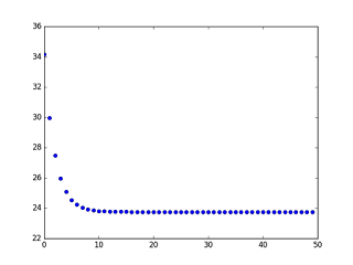
As you see in the graph error function is diminishing at each run. But by time
improvement is getting smaller.

for learning_rate = 0.001
It seems it is learning faster. But be careful this is a simple example and our distribution is simple with only one minimum.
If we had a complex function who has lots of convex ,concave shapes then our high/low learning rates could skip global minimum
or stuck in local minimum. Check pictures in net for these effects. There are lots of nice pictures.

You can play with parameters below and you will obtain very different results according to your parameters.

num_tests = 10
mycoef = 1
iter_count = 500

learning_rate = 0.001
initial_b = 0 # initial y-intercept guess
initial_m = 0 # initial slope guess


figError, axError = plt.subplots()

fig2, ax2 = plt.subplots()
plt.figure(1)

ax2.plot(x1, y1, 'ro')

errorList = [];


for i in range(num_tests):
  [b, m] = gradient_descent_runner(points, initial_b, initial_m, learning_rate, (i+mycoef)* iter_count)  
  
  
  x = np.linspace(0, 50, 49)
  y = x *m + b
  ax2.plot(x, y, 'k--')
  ax2.text(max(x),max(y),i)

  error = compute_error_for_line_given_points(b, m, points)
  errorList.append( error );
  
  
  axError.plot( i ,error , 'bo')
  print "After {0} iterations b = {1}, m = {2}, error = {3}".format( (i+mycoef)* iter_count, b, m, error)

Below is a result of parameters
num_tests = 10
mycoef = 1
iter_count = 500

You can play as much as you want and see the of error, slope and intercept.
Below graph seems bad because ,function performs so good from beginning and lines overlap.

Part I took from article

from numpy import *
import numpy as np
from StringIO import StringIO
import matplotlib.pyplot as plt
import numpy as np

# y = mx + b
# m is slope, b is y-intercept
def compute_error_for_line_given_points(b, m, points):
    totalError = 0
    for i in range(0, len(points)):
        x = points[i][ 0]
        y = points[i][ 1]
        totalError += (y - (m * x + b)) ** 2
    return totalError / float(len(points))

def step_gradient(b_current, m_current, points, learningRate):
    b_gradient = 0
    m_gradient = 0
    N = float(len(points))
    for i in range(0, len(points)):
        x = points[i, 0]
        y = points[i, 1]
        b_gradient += -(2/N) * (y - ((m_current * x) + b_current))
        m_gradient += -(2/N) * x * (y - ((m_current * x) + b_current))
    new_b = b_current - (learningRate * b_gradient)
    new_m = m_current - (learningRate * m_gradient)
    return [new_b, new_m]

def gradient_descent_runner(points, starting_b, starting_m, learning_rate, num_iterations):
    b = starting_b
    m = starting_m
    for i in range(num_iterations):
        b, m = step_gradient(b, m, array(points), learning_rate)
    return [b, m]